Enhancing Monocular Metric Depth Estimation through Adaptive Scaling
This page is based on the following resources:
Report
Poster
Code
Introduction
Monocular depth estimation (MDE) is a core task in computer vision with applications in autonomous driving, robotics, and augmented reality (AR) [1][2]. Despite advances in deep learning, predicting metric depth from a single image remains difficult due to scale ambiguity — the loss of absolute scale during perspective projection [3][4]. This limits real-world deployment in tasks like robot navigation and 3D reconstruction [5].
Most MDE models predict relative depth, learning ordinal relationships without recovering true scale [6]. Some methods use LiDAR [7], stereo vision [8], or geometric self-supervision [9], but these approaches add complexity or lack generalization. Others assume fixed depth ranges [10], which fail across diverse scenes.
Recent efforts introduce learned scale factors [10], depth priors [11], or motion cues [12], but often lack robustness in unfamiliar environments.
We address this with a lightweight adaptive scaling framework that predicts an image-specific depth scaling factor, enabling accurate metric depth estimation without extra sensors or manual tuning. Our pipeline involves:
- Generating optimal scaling factors by minimizing scale-invariant error between predicted and ground-truth depth maps from NYU Depth V2, using Depth Anything V2 as the base predictor [10].
- Training a lightweight CNN to predict these scale corrections directly from RGB images.
Our method improves monocular depth estimation across metrics like AbsRel, RMSE, and δ₁ accuracy, enhancing reliability in real-world robotics, AR, and scene understanding.
Method
Generating Optimal Scaling Factors
We first examine Depth Anything V2 [10], a state-of-the-art monocular depth estimation model, on the NYU Depth V2 dataset to evaluate its metric depth estimation performance. As illustrated in Fig. 1, the model produces depth maps whose distributions closely resemble the ground truth, indicating accurate prediction of relative depth.
However, despite this structural similarity, the predicted maps consistently exhibit linear scale discrepancies when compared to ground truth, highlighting the classic scale ambiguity challenge in monocular depth estimation.
This observation motivated our core hypothesis: that learning to predict an image-specific scaling factor could substantially improve the metric accuracy of monocular depth predictions, without modifying the base model or requiring extra sensors.
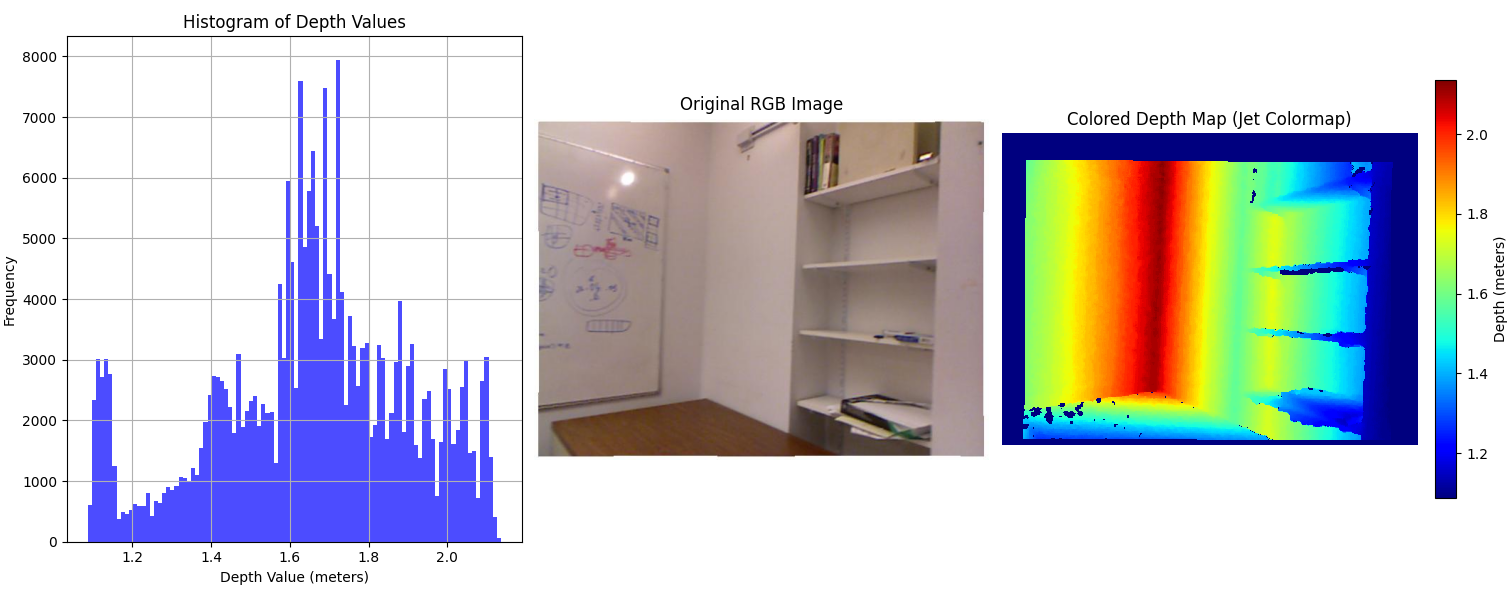
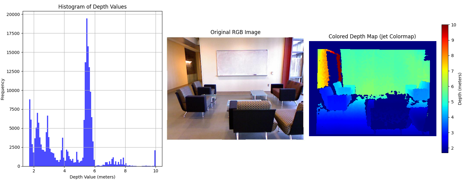
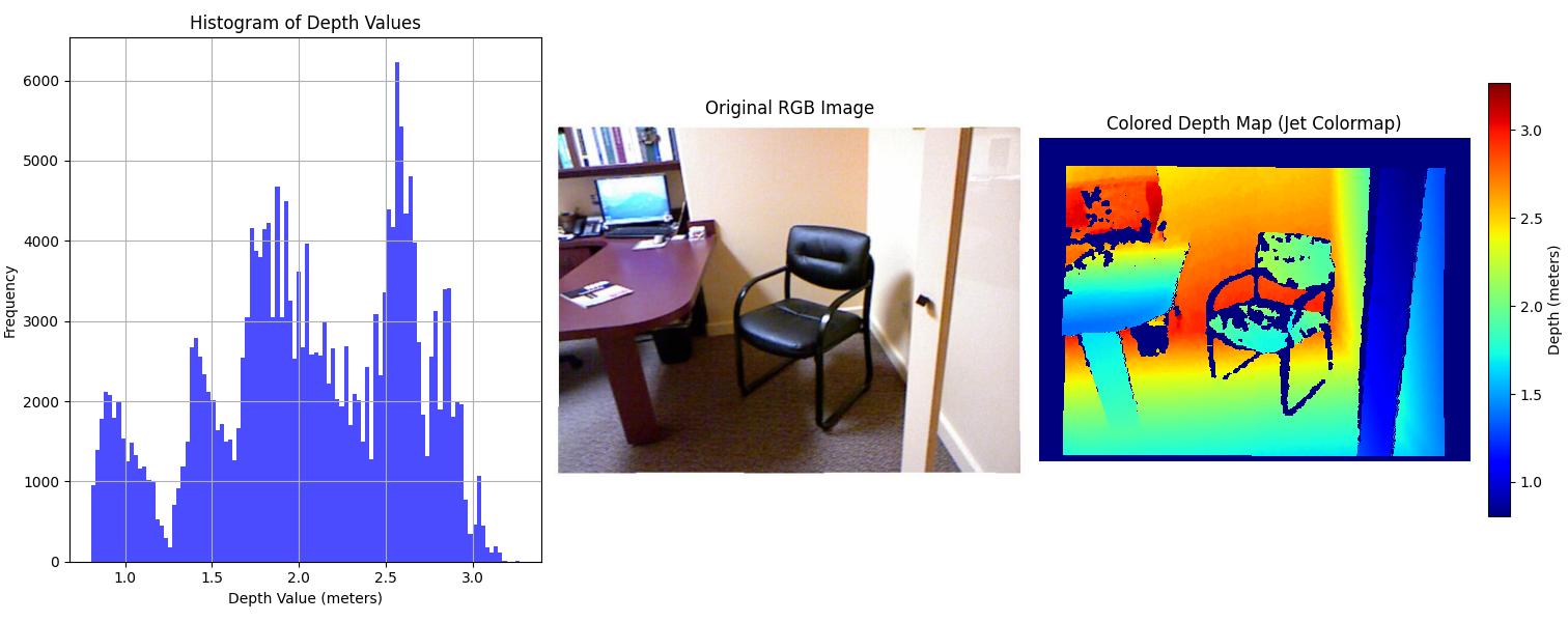
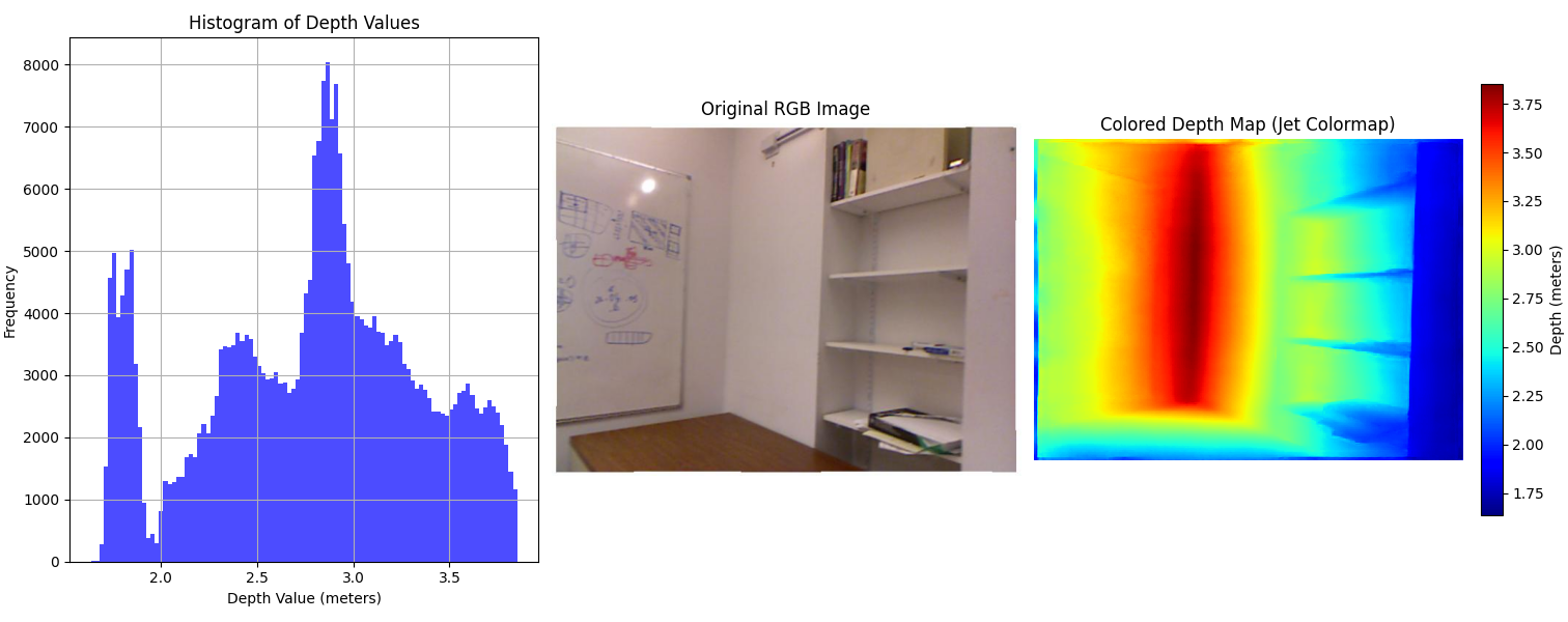
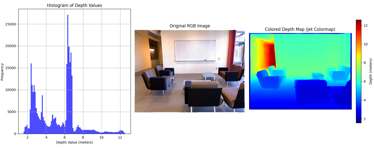
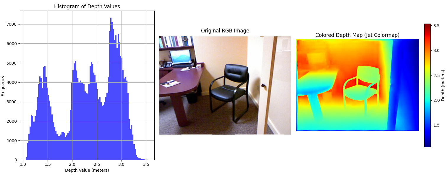
Fig. 1: Top: Ground truth depth maps. Bottom: Depth Anything V2 predictions. Scale discrepancies in the predicted maps are clearly visible.
To correct these predictions, we compute an optimal scaling factor for each image that aligns the predicted and ground-truth depth distributions by minimizing the Wasserstein distance. The Wasserstein distance (also known as Earth Mover’s Distance) measures the minimum “effort” required to transform one distribution into another — making it a natural choice for aligning depth histograms, where the goal is to correct global scale without distorting the underlying structure. This formulation allows us to find the scale that best matches the predicted depth distribution to the ground truth:
\[ s^* = \underset{s \in [0.1, 2.0]}{\arg\min} \, W(s \cdot D_{\text{pred}}, D_{\text{gt}}) \]
Here, \( s^* \) denotes the optimal scaling factor, \( D_{\text{pred}} \) is the predicted depth map generated by Depth Anything V2, and \( D_{\text{gt}} \) represents the ground truth depth map. The function \( W \) refers to the Wasserstein distance, capturing the global discrepancy between the two distributions.
This optimization is solved per image over 392 RGB-depth pairs from NYU Depth V2 [13]. The resulting scale factors are log-transformed for stability and used to create a supervised dataset for training a neural network.
Training a Depth Scaling Predictor
To enable scale correction at test time, we train a lightweight convolutional neural network (CNN) that predicts the log of the optimal scaling factor directly from an input RGB image.
This model is intentionally kept small to ensure fast inference and ease of integration into existing monocular depth pipelines. Since the scaling factor is a global property of the image, the task does not require complex spatial reasoning or deep feature hierarchies — making a shallow CNN both effective and efficient.
CNN Architecture
The network consists of two convolutional layers with 64 and 128 channels, each followed by ReLU activation and max pooling. The resulting feature map is flattened and passed through a fully connected layer with 512 units, followed by a final linear layer that outputs a single log-scale value per image.
Training Configuration
The model is trained on 392 RGB images from NYU Depth V2 [13], each labeled with a log-transformed optimal scaling factor computed during preprocessing.
- Loss Function: Mean Squared Error (MSE) between predicted and ground-truth log-scales
- Optimizer: Adam with a learning rate of \(10^{-3}\), using step decay every 10 epochs
- Training Duration: 30 epochs
- Validation: Evaluated every 5 epochs on a 20% validation split
- Batch Size: 30
Experimental Results
We evaluate our adaptive scaling method by comparing it against two baselines:
(1) the unscaled predictions from Depth Anything V2 (DA2), and
(2) predictions refined using ground-truth optimal scaling factors obtained via offline optimization.
Our evaluation covers both quantitative metrics and qualitative visualizations, including:
- Training and validation loss curves to demonstrate convergence
- Accuracy of predicted scaling factors on training and test splits
- Depth estimation performance using AbsRel, RMSE, and δ₁ metrics
- Point cloud reconstructions highlighting geometric improvements
Training and Validation Loss
We begin by analyzing the training dynamics of the scaling predictor. As shown in Fig. 2, the training and validation losses decrease rapidly during the early stages and gradually stabilize, indicating consistent learning and convergence. The use of log-scaled loss visualization reveals smooth convergence behavior.
Notably, the validation loss closely follows the training loss across epochs, occasionally dipping below it — a sign of good generalization without significant overfitting.
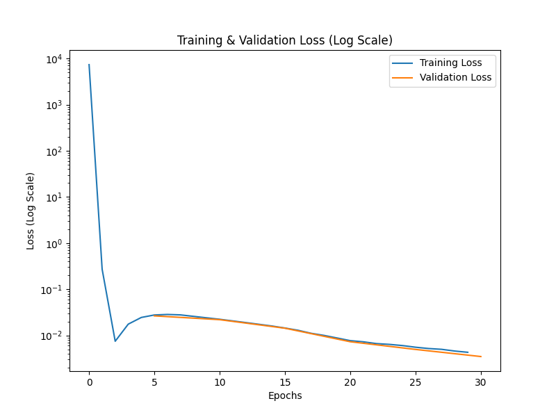
Fig. 2: Training and validation loss curves (log scale). The model converges stably and generalizes well across epochs.
Scaling Factor Prediction Accuracy
We first evaluate the CNN’s ability to estimate log-scale factors on both the training and test splits. The results, shown in Table 1, report mean absolute error (MAE) and root mean squared error (RMSE) between predicted and ground-truth log-scales.
| Dataset | MAE ↓ | RMSE ↓ |
|---|---|---|
| Training Set | 0.0439 | 0.0532 |
| Test Set | 0.1172 | 0.1269 |
These results show that our lightweight CNN effectively learns to predict image-conditioned scaling factors, achieving low error rates on the training set and reasonable generalization to unseen data. While errors increase slightly on the test set (as expected from domain variation), the model consistently captures the global relationship between image features and scale.
Depth Estimation Performance
We evaluate depth prediction accuracy across three settings:
- DA2 w/o scaling (baseline),
- DA2 w/ oracle scale (ground-truth scaling factor), and
- DA2 w/ adaptive scale (ours).
We report three widely-used metrics:
-
Absolute Relative Error (AbsRel):
\[ \text{AbsRel} = \frac{1}{N} \sum_{i=1}^{N} \frac{|D_i^{\text{pred}} - D_i^{\text{gt}}|}{D_i^{\text{gt}}} \]
Captures average relative error across pixels. -
Root Mean Squared Error (RMSE):
\[ \text{RMSE} = \sqrt{\frac{1}{N} \sum_{i=1}^{N} (D_i^{\text{pred}} - D_i^{\text{gt}})^2} \]
Penalizes larger errors more heavily. -
Threshold Accuracy (δ₁):
\[ \delta_1 = \frac{1}{N} \sum_{i=1}^{N} \mathbb{1} \left( \max\left( \frac{D_i^{\text{pred}}}{D_i^{\text{gt}}}, \frac{D_i^{\text{gt}}}{D_i^{\text{pred}}} \right) < 1.25 \right) \]
Measures the percentage of predictions within a 25% range of the ground truth.
Results on both training and test sets are summarized in Table 2:
| Method | AbsRel ↓ | RMSE ↓ | δ₁ (%) ↑ |
|---|---|---|---|
| Training Set | |||
| DA2 w/o scaling | 0.2219 | 0.9480 | 66.82 |
| DA2 w/ Oracle Scale | 0.0554 | 0.3083 | 93.87 |
| DA2 w/ Adaptive Scale (Ours) | 0.0792 | 0.3632 | 96.07 |
| Test Set | |||
| DA2 w/o scaling | 0.3380 | 0.6166 | 32.06 |
| DA2 w/ Oracle Scale | 0.1084 | 0.2307 | 87.94 |
| DA2 w/ Adaptive Scale (Ours) | 0.1914 | 0.3636 | 72.31 |
These results confirm that our adaptive scaling approach significantly improves depth estimation accuracy over the unscaled baseline. On the training set, our method reduces AbsRel from 0.2219 to 0.0792 and boosts δ₁ from 66.82% to 96.07%, even surpassing the oracle in pixel-wise agreement. On the test set, while a gap remains between adaptive and oracle scaling, our model still achieves substantial gains — reducing AbsRel by 43% and more than doubling δ₁ accuracy from the unscaled baseline.
Point Cloud Comparisons
To further evaluate the effectiveness of our adaptive scaling method, we visualize 3D point clouds reconstructed from the predicted depth maps. These qualitative results highlight the geometric improvements achieved through scale correction.
In Fig. 3, we compare point clouds generated from:
- Oracle-scaled predictions (green),
- Predictions scaled using our adaptive CNN (blue), and
- Unscaled DA2 predictions (red),
each overlaid with the ground truth point cloud for reference.
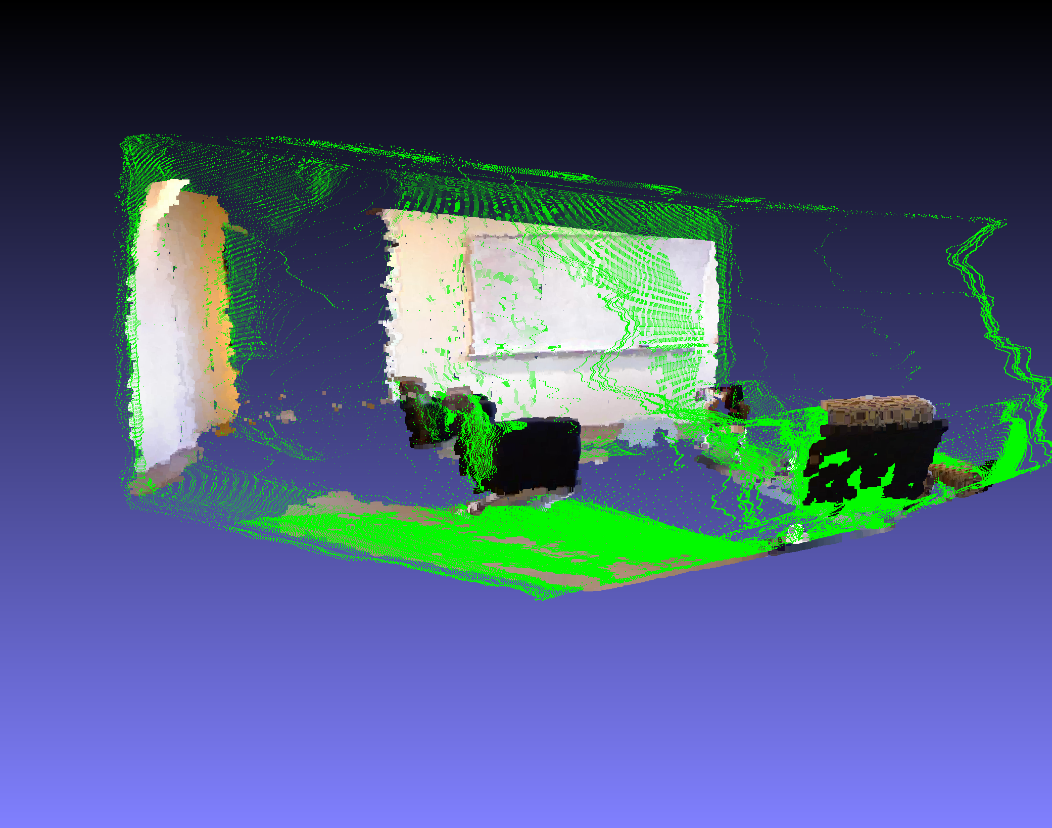
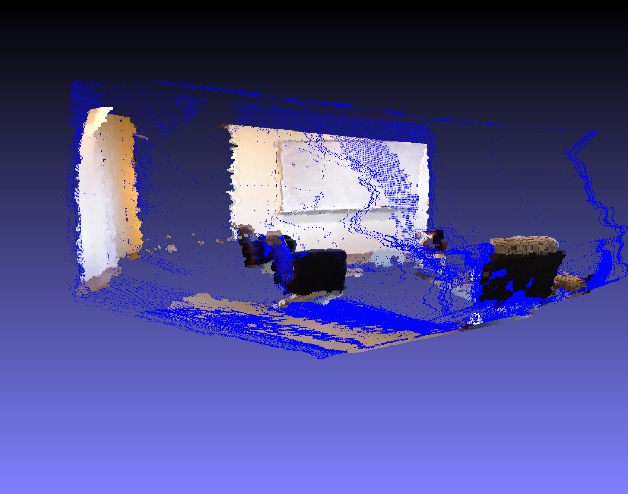
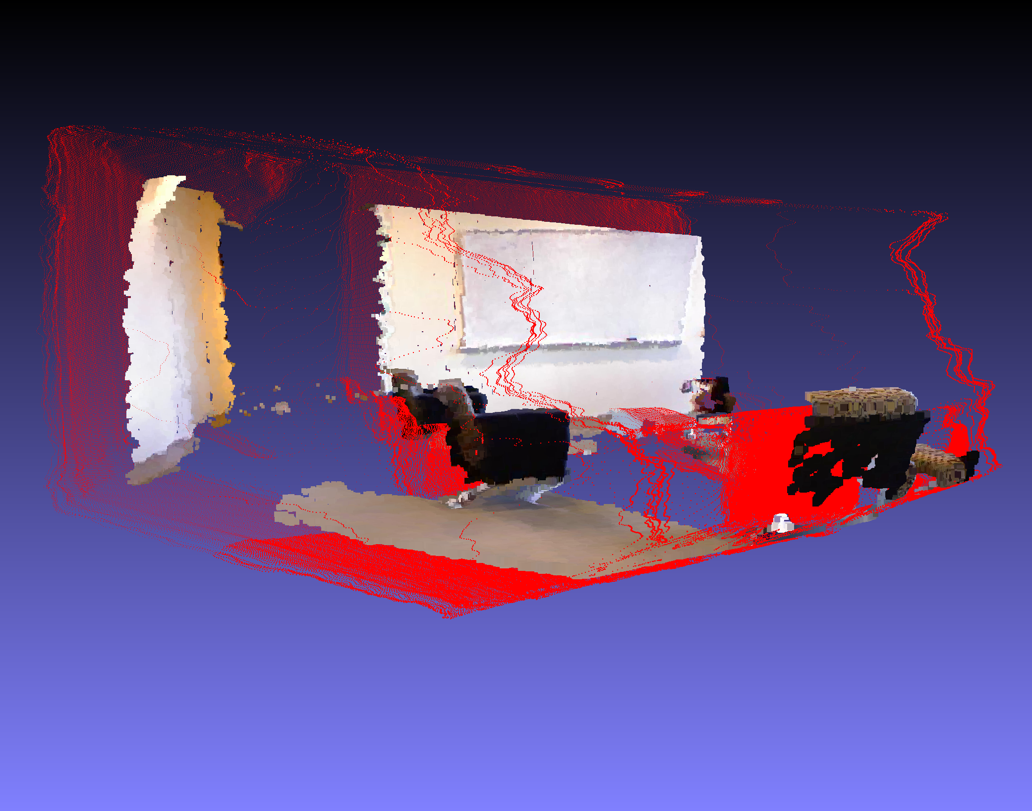
Fig. 3: 3D point cloud comparisons. Left: Oracle-scaled prediction (green). Middle: Adaptive scaled prediction (blue). Right: Unscaled DA2 prediction (red). Ground truth point clouds are shown for reference in all plots.
The unscaled predictions (right) result in distorted and misaligned 3D reconstructions due to incorrect global scale. In contrast, the adaptive scaled output (middle) shows significantly better alignment with the ground truth geometry — closely approaching the oracle-scaled performance (left).
Conclusion
In this project, we addressed a fundamental limitation in monocular depth estimation: the inability to recover consistent metric scale from single RGB images. While state-of-the-art models like Depth Anything V2 excel at predicting relative depth, they often fail to generalize metric accuracy across diverse environments due to scale ambiguity.
We proposed a lightweight, sensor-free framework that learns an image-conditioned scaling factor to correct global scale errors in monocular depth maps. Our method requires no modifications to the underlying depth model and can be integrated as a post-processing step.
Through both quantitative metrics and qualitative 3D visualizations, we demonstrated that our adaptive scaling approach:
- Significantly reduces depth estimation error over baseline predictions,
- Generalizes reasonably to unseen test scenes, and
- Produces geometrically consistent point clouds close to oracle-scaled results.
This validates our core hypothesis: learning global scaling from image features alone is both feasible and effective for improving metric depth estimation.
Future Work
To further improve the robustness and versatility of our method, future work will focus on two directions. First, we aim to develop a mechanism to detect erroneous depth predictions prior to inference, enabling selective correction and improving overall reliability. Second, we plan to extend our framework to support pixel-wise adaptive scaling, allowing it to handle complex scenes with depth discontinuities and spatially varying scale — such as indoor environments with occlusions, reflective surfaces, or large open spaces.
References
[1] R. Ranftl et al., “Towards robust monocular depth estimation,” NeurIPS, 2022.
[2] W. Yin et al., “Geometric structure preserving depth estimation,” CVPR, 2023.
[3] D. Eigen et al., “Depth map prediction from a single image,” NeurIPS, 2014.
[4] J.-W. Bian et al., “Unsupervised scale-consistent depth and ego-motion,” NeurIPS, 2019.
[5] C. Godard et al., “Digging into self-supervised monocular depth estimation,” ICCV, 2019.
[6] R. Ranftl et al., “MiDaS v3: Monocular depth estimation,” arXiv, 2023.
[7] R. Wang et al., “LiDAR-augmented monocular depth estimation,” CVPR, 2021.
[8] B. Ummenhofer et al., “DeMoN: Depth and motion network,” CVPR, 2017.
[9] J. Watson et al., “Temporal self-supervision for monocular 3D detection,” NeurIPS, 2021.
[10] X. Li et al., “Depth Anything V2,” arXiv, 2024.
[11] T. Zhou et al., “Unsupervised learning of depth and ego-motion,” CVPR, 2017.
[12] Y. Zhou et al., “Adaptive scaling for depth estimation with motion cues,” CVPR, 2023.
[13] N. Silberman et al., “Indoor segmentation and support inference from RGB-D,” ECCV, 2012.
